Rasterization on Larrabee

https://software.intel.com/en-us/articles/rasterization-on-larrabee

— 翻译:　Yongjiu Wei 2015/07/25 05:32

Rasterization on Larrabee

注: Larrabee 是英特尔公司的通用图形处理器（GPCPU）的开发代号/核心代号, 详见Larrabee

By Michael Abrash

You don't tug on Superman's cape

You don't spit into the wind

You don't pull the mask off that old Lone Ranger

And you don't mess around with Jim

以上为歌曲《You Don't Mess Around with Jim》的部分歌词

The first time you heard the chorus of “You Don't Mess Around with Jim,” you no doubt immediately wondered why Jim Croce left out: “And you don't rasterize in software if you're trying to do GPU-class graphics, even on a high-performance part such as Larrabee.” That's just common sense, right? It was obvious to me, anyway, that Larrabee was going to need a hardware rasterizer. But maybe Jim knew something I didn't, because it turned out I was wrong, and therein lies a tale.

第一次听到“你别和 Jim 混混” 时你肯定好奇为什么 Jim Croce 遗漏了这句 “如果你做GPU,就不需要软件光栅化, 即使是在高性能的 Larrabee 上”, 这是常识啊, 不是么? 对我而言, 显然, 至少 Larrabee 要上硬件光栅. 但可能 Jim 知道些我不知道的东西, 因为结果显示我是错的, 这里面有些故事.

First, though, let's back up a step and get some context.

但首先, 我们回退一步交代些背景.

半并行任务的并行设计

Last month, in “A First Look at the Larrabee New Instructions (LRBni),” we got an overview of Larrabee, an upcoming multi-threaded, vectorized, many-core processor from Intel. It may not be entirely apparent from last month's whirlwind tour, but the Larrabee New Instructions contains everything you need to do a great job running code that's designed to be vectorized, such as HLSL shaders. But what about tasks that aren't inherently scalar (in particular, where the iterations aren't serially dependent), but that at the same time can't be efficiently parallelized in any obvious way, and for which the usual algorithms aren't easily vectorized?

上月, 在“Larrabee新指令集预览”里我们获知了 Larrabee 的概况: 一个即将到来的支持多线程,矢量化的英特尔多核处理器. 上月一连串宣讲可能并不完整展现 Larrabee, 但新指令集 Larrabee 包含了所有你做那些矢量化运行代码的重大任务时需要的事物, 比如 HLSL 着色器. 但是那些非固有标量又同时不能明显并行化的任务, 以及不容易矢量化的常见算法要怎么办呢?

In the process of implementing the standard graphics pipeline for Larrabee, we (the Larrabee team at RAD: Atman Binstock, Tom Forsyth, Mike Sartain, and I) have gotten considerable insight into that question, because while the pipeline is largely vectorizable, there are a few areas in which the conventional approaches are scalar, and where some degree of serialization is unavoidable. This article will take a close look at how we applied the Larrabee New Instructions to one of those problem areas, rasterization, in the process redesigning our implementation so it was far more vectorizable, and also so it took advantage of the strengths of Larrabee's CPU-based architecture. Needless to say, performance with the Larrabee New Instructions will vary greatly from one application to the next - there's not much to be done with purely scalar code - but diving into Larrabee rasterization in detail will give a good sense for what it's like to apply the Larrabee New Instructions to at least one sort of non-obvious application.

在Larrabee 标准图形管线的实现过程中, 我们( RAD 的Larrabee 团队: Atman Binstock, Tom Forsyth, Mike Sartain, 和我)已经对此问题有相当多的考虑, 因为尽管大部分管道可以矢量化,但还是有小部分地方的常规处理方法是标量的,某些程度的序列化是不可避免的.本文将仔细讲解我们怎么应用新指令集Larrabee来处理这些问题之一: 光栅化, 通过重设计实现来让它更为矢量化, 更贴合Larrabee基于CPU的架构的优势特点.不用说, 新指令集Larrabee的在序列应用上的表现是很出色的, 纯标量代码上是不需要多说的,但深入到新指令集Larrabee的细节, 可以很好得感受新指令集Larrabee处理那一类特殊应用时的样子.

Before we begin, in order to avoid potential confusion, let me define “rasterization”: for our present purposes, it's the process of determining which pixels are inside a triangle, and nothing more. In this article, I won't discuss other aspects of the rendering pipeline, such as depth, stencil, shading, or blending, in any detail.

在开始之前, 为了避免可能的困扰, 让我们来定义下“光栅化”:从我们的目的来看, 它是一个决定哪些像素在一个三角形内的过程,仅此而已. 在这篇文章中, 我不会讨论渲染管线上的其它方面, 比如深度, 模板, 着色, 混色等细节.

光栅化曾是个爱惹麻烦的孩子 - 但麻烦比我们所想的要少

When we look at applying the Larrabee New Instructions to the graphics pipeline, for the most part it's easy to find 16-wide work for the vector unit to do. Depth, stencil, pixel shading, and blending all fall out of processing 4×4 blocks, with writemasking at the edges of triangles. Vertex shading is not quite a perfect fit, but 16 vertices can be shaded and cached in parallel, which works well because vertex usage tends to be localized. Setting up 16 triangles at a time also works pretty well; there's some efficiency loss due to culling, but it still yields more than half of maximum parallelism.

当我们审视 LNI 在图形管道上的应用时, 很容易发现大部分范围在做矢量单位16位宽的操作. 景深, 模板, 像素着色, 与色混合, 都会归结为 4×4 块的操作, 伴随三角形边的写屏蔽操作( writemasking:?:). 这并不完全适用于顶点着色, 但 16 个顶点可被很好得并行着色与储存, 因为顶点趋向于局部被使用. 同时组建 16 个三角形也可以很好得运行; 虽然有一些剪裁导致的性能损失, 但它仍然有最大并行一半以上的收益.

That leaves rasterization, which is definitely not easy to vectorize with good enough performance to be competitive with hardware. As an aside, the Larrabee rasterizer is not, of course, the only rasterizer that could be written for Larrabee. There are other rasterizers for points and lines, and of course there may be other future rasterizers for interesting new primitive types. In fact, I suggest you write your own - it's an interesting problem! But as it doesn't have a more formal name, I'll just refer to the current general-purpose triangle rasterizer as “the Larrabee rasterizer” in this article.

最后还有光栅化, 相比硬件, 光栅化肯定不容易得到足够竞争性能的矢量化. 题外话, Larrabee 的(三角形)光栅器当然不是唯一在 Larrabee 上可写的光栅器. 有其它点与面的光栅器, 当然还可能有其它有趣的新原生类型的未来光栅器. 事实上, 我建议你自己写一个 - 这很有趣! 由于没有一个更正规的名字, 在本文中我会把当前通用的三角形光栅器称作 Larrabee 光栅器.

The Larrabee rasterizer was at least the fifth major rasterizer I've written, but while the others were loosely related, the Larrabee rasterizer belongs to a whole different branch of the family - so different, in fact, that it almost didn't get written. Why not? Because, as is so often the case, I wanted to stick with the mental model I already understood and was comfortable with, rather than reexamining my assumptions. Long-time readers will recall my fondness for the phrase “Assume nothing”; unfortunately, I assumed quite a lot in this case, proving once again that it's easier to dispense wise philosophy than to put it into action!

Larrabee 光栅器是我写过的至少第五个主要光栅器, 虽然与其它光栅器有松散的关系, 但 Larrabee 光栅器仍可属于该家族的一个完全不同的分支 - 事实上,由于那么不同, 它差点没被写出来. 为什么写不出来? 因为 - 这种情况比较常见 - 我想继续跟着我已经理解的思维模式, 这比重新审视自己的设想要来得舒服. 老读者会想起我钟爱于这个短语“不做任何的假设”; 不幸的是, 这次我做了许多假设, 再一次证明人生哲学说起来比践行容易.

Coming up with better solutions is all about trying out different mental models to see what you might be missing, a point perfectly illustrated by my efforts about 10 years ago to speed up a texture mapper. I had thrown a lot of tricks at it and had made it a lot faster, and figured I was done; but just to make sure, I ran it by my friend David Stafford, an excellent optimizer. David said he'd think about it, and would let me know if he came up with anything.

更好的解决方案的出现, 完全是尝试不同的思维模式以找出你可能错过的东西, 我十年前对加速纹理映射所做的努力可以完美诠释这个观点. 为了让纹理映射器更加快, 我曾抛弃了许多把戏并以为做到足够了, 但为了确定, 我让我的朋友 David Stafford , 一个卓越的优化者, 跑跑它. David 说他会仔细考虑, 有什么想法时再告诉我.

When I got home that evening, there was a message on the answering machine from David, saying that he had gotten 2 cycles out of the inner loop. (It's been a long time, and my memories have faded, so it may not have been exactly 2 cycles, but you get the idea.) I called him back, but he wasn't home (this was before cellphones were widespread). So all that evening I tried to figure out how David could have gotten those 2 cycles. As I ate dinner I wondered; as I brushed my teeth I wondered; and as I lay there in bed not sleeping, I wondered. Finally I had an idea - but it only saved 1 cycle, not 2. And no matter how much longer I racked my brains, I couldn't get that second cycle.

当天晚上我到家后, David 就来了一个消息(估计是BP机), 说他把内循环减少了两个周期. (时间比较久远了, 记忆模糊, 所以可能不是精确的两个周期, 但你懂的) 我打电话给他, 但他不在家 ( 那时手机还没普及). 所以整个晚上我试图找出 David 优化的那两个循环. 我吃晚饭时想, 我刷牙时想, 我躺在床上想着睡不着. 最后我有了一个主意 - 但它只节约了一个循环, 不是两个. 不管我怎么绞尽脑汁, 我搞不到第二个循环.

The next morning, I called David, admitted that I couldn't match his solution, and asked what it was. To which he replied: “Oh, sorry, it turned out my code doesn't work.”

第二天早上, 我承认了自己找不出他的优化方式, 打电话给 DaviD 询问. 他回复:“哦, 抱歉, 最后才发现我那代码不起作用.”

It's certainly a funny story, but, more to the point, the only thing keeping my code from getting faster had been my conviction that there were no better solutions - that my current mental model was correct and complete. After all, the only thing that changed between the original solution and the better one was that I acquired the belief that there was a better solution - that is, that there was a better model than my current one. As soon as I had to throw away my original model, I had a breakthrough.

这是个相当有趣的故事, 但, 更多的是指出唯一让我代码不能更快的是我对没有更好解决办法的自信 - 我的思维模式是正确完美的. 归根结底, 原来的解决方案与更好的解决方案之间唯一改变的事情是我确信了有一种更好的解决方案 - 那就是, 有一种比我当前更好的方式. 一旦我抛弃了原来的思考模式, 我就有了一个更好的突破.

Software rasterization was a lot like that.

软件光栅化也类似这个.

The previous experience that Tom Forsyth and I had had with software rasterization was that it was much, much slower than hardware. Furthermore, there was no way we could think of to add new instructions to speed up the familiar software rasterization approaches, and no obvious way to vectorize the process, so we concluded that a hardware rasterizer would be required. However, this turned out to a fine example of the importance of reexamining assumptions.

以前 Tom Forsyth 和我在软件光栅化上的经验就是它比硬件要慢, 慢得多. 此外, 我们想不出一个办法来添加新指令集来加速软件光栅化, 也想不出一个明显的路子来让过程向量化, 所以我们得出必须有硬件光栅器的结论. 然而, 这变成了重新检验设想的重要性的一个很好的例子.

In the early days of the project, as the vector width and the core architecture were constantly changing, one of the hardware architects, Eric Sprangle, kept asking us whether it might be possible to rasterize efficiently in software using vector processing, and we kept patiently explaining that it wasn't. Then, one day, he said: “So now that we're using the P54C core, do you think software rasterization might work?” To be honest, we thought this was a pretty dumb question, since the core didn't have any significant impact on vector performance; in fact, we were finally irritated enough to sit down to prove in detail - with code - that it wouldn't work.

在项目早期, 由于矢量宽度和核心架构持续在改变, 一个硬件设计师 Eric Sprangle 一直在问我们是否有可能利用矢量处理来高性能得进行软件光栅化, 我们一直耐心得解释那不可能. 有一天, 他说:“现在我们在用 P54C 核, 你觉得软件光栅化能行了么? ” 说实话, 我们认为这是很人无语的问题, 因为那个核没有任何矢量性能上的重要影响; 实际上, 我们最终恼怒得坐下来用代码来详细证明它不可行.

And we immediately failed. As soon as we had to think hard about how the inner loop could be structured with vector instructions, and wrote down the numbers - that is, as soon as our mental model was forced to deal with reality - it became clear that software rasterization was in fact within the performance ballpark. After that it was just engineering, much of which we'll see shortly.

我们立刻失败了. 一旦我们必须努力去想如何让内循环满足矢量运算指令并写数字 – 那就是, 一旦我们的思考模式被迫去考虑处理实际情形 – 就会清晰发现软件光栅化实质也处在性能优化领域中. 然后这就仅仅是工程问题, 其中大部分我们就要讲到.

First, though, it's worth pointing out that, in general, dedicated hardware will be able to perform any specific task more efficiently than software; this is true by definition, since dedicated hardware requires no multifunction capability, so in the limit it can be like a general-purpose core with the extraneous parts removed. However, by the same token, hardware lacks the flexibility of CPUs, and that flexibility can allow CPUs to close some or all of the performance gap. Hardware needs worst-case capacity for each component, so it often sits at least partly idle; CPUs, on the other hand, can just switch to doing something different, so ALUs are never idle. CPUs can also implement flexible, adaptive approaches, and that can make a big difference, as we'll see shortly.

然而首先, 值得指出, 大致上, 专用硬件执行具体任务都会比软件性能要高; 这很显然, 因为专用硬件不需要多功能, 严格来说它就像一个通用核去掉了外部部分. 然而, 同样的, 硬件缺乏 CPU 的灵活性, 这种灵活性能让 CPU 规避部分或全部性能缺口. 硬件需要每个零件在最坏情形下的性能, 所以它经常处于某种程度上的空转; 另一方面, CPU 则可以直接切换去干其他事情, ALU(Arithmetic Logic Unit, 算术逻辑单元是中央处理器的执行单元，是所有中央处理器的核心组成部分) 永远不会空转. CPU 也能实现灵活适用的手段, 这些手段之间差异很大, 我们马上会讲到.

为什么光栅化曾是个爱惹麻烦的孩子

I can't do a proper tutorial on rasterization here, so I'll just run through a brief refresher. For our purposes, all rasterization will be of triangles. There are three edges per triangle, each defined by an equation Bx+Cy relative to any point on the edge, with the sign indicating whether a point is inside or outside the edge. Both x and y are in 15.8 fixed-point format, with a range of [-16K, +16K). The edge equations are tested at pixel or sample centers, and for cases where a pixel or sample center is right on an edge, well-defined fill rules must be observed (in this case, top-left fill rules, which are generally implemented by subtracting 1 from the edge equation for left edges and flat top edges). Rasterization is performed with discrete math, and must be exact, so there must be enough bits to represent the edge equation completely. Finally, multisampled antialising must be supported.

我不能在这里做个光栅化的正式说明, 所以我只做个简要的复习. 基于我们的目的, 所有光栅化都是关于三角形的. 每个三角形有三条边, 每条边由二维方程式 Bx+Cy 定义有哪些点在边上, 以及在边内还是在边外的标志. x 和 y 都是 15.8 定点格式, 范围为 [-16K, +16K). 边的方程式被用来测试像素点或样本中心点, 为方便判断哪些像素或样本中心点在边上, 必须要有一个定义好的填充规则 (在这个例子中为 top-left 填充规则, 此规则一般对上方与左方的边减 1 ). 光栅化的执行靠离散数学, 并要求准确, 所以必须有足够的位来完全表现边方程式. 最后, 多样本反锯齿(译者: Multisampled Anti-alising)也必须支持.

Let's look at a quick example of applying the edge equation. Figure 1 shows an edge from (12, 8) to (4, 24). The B coefficient of the edge equation is simply the edge's y length: (y1 - y0). The C coefficient is the negation of the edge's x length: (x0 - x1). Thus, the edge equation in Figure 1 is (24 - 8)x + (12 - 4 )y. Since we only care about the sign of the result (which indicates inside or outside), not the magnitude, this can be simplified to 2x + 1y, where the x value used in the equation is the distance between the point of interest and any point at which the equation is known to be zero (which is to say any point on the line); usually a vertex is used, as for example the vertex at (12, 8) is used in Figure 1. All points on the edge have the value 0, as can be seen in Figure 1 for the point on the line at (8, 16).

让我们来看看一个应用边方程式的简要例子. 图例 1 显示了一条从 (12, 8) 到 (4, 24)的边. 边方程式的 B 系数 就是边的 y 的长度: (y1 - y0). C 系数则是边 x 的长度的负数: (x0 - x1). 这样, 图例 1 中的边方程式就是 (24 - 8)x + (12 - 4)y. 由于我们只关心结果(在里面还是在外面), 不关心量级, 所以方程式可简化为 2x + 1y, 这里 x 的值就是所测的点与方程值为 0 时的点(可以说该线条上的任意点)之间的相对距离; 通常会使用(三角形的)顶点, 比如图例 1 中的 (12, 8) 的顶点. 所有在边上的点的值为0, 比如图例 1 中的 (8, 16).

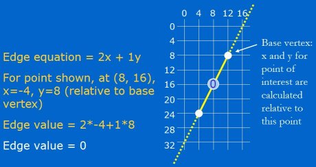
Figure 1: Points on an edge always have an edge equation value of zero.

图例 1 :　在边上的点的边方程式的值总为 0.

Points on one side of the edge will have positive values, as shown in Figure 2 for the point at (12, 16), which has a value of 8.

在边的其中一边方向的点会是正值, 比如图例 2 中的点 (12, 16), 它的值为 8.

Figure 2: Points on one side of an edge are always positive.

图例 2 在边的其中一边方向的点都是正值.

Points on the other side of the edge will have negative values, as shown in Figure 3 for the point at (4, 12), which has a value of -12.

在另外一边方向上的点都会是负值, 比如图例 3 的点(4, 12), 它的值为 -12.

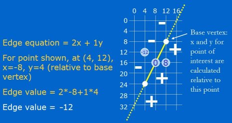
Figure 3: Points on the other side of the edge are always negative.

图例 3 在另外一边方向上的点都会是负值.

Simple though it is, the edge equation is the basis upon which the Larrabee rasterizer is built. By applying the three edge equations at once, it is possible to determine which points are inside a triangle, and which are not. Figure 4 shows an example of how this works; the pixels shown in green are considered to be inside the triangle formed by the edges, because their centers are inside all three edges. As you can see, the edge equation is negative on the side of each edge that's inside the triangle; in fact, it gets more negative the farther you get from the edge on the inside, and more positive the farther you get from the edge on the outside.

简单考虑, Larrabee 光栅化就是在边方程式基础上计算的.一次性计算三个边方程式, 就能决定哪些点位于在三角形内, 哪些点在外. 图例 4 展示了一个如何计算的例子; 绿色的像素点被认为是在三角形内, 因为它们的中心点在三条边之内.如你所见, 每条边方程式均为负值即在三角形内部. 实际上, 内部离边越远所得负值越大(译者: 指绝对值越大), 外部离边越远所得正值越大.

Figure 4: Rasterization of a triangle, defined by three edges, each with an inside (negative edge equation values) and an outside (positive edge equation values). Pixels are categorized as inside or outside based on edge equation values at pixel centers (white dots).

图例 4 三角形的光栅化, 三角形三条边, 每条边区分了内部(边方程式值为负)与外部(边方程式值为正). 像素点归类为内部点还是外部点基于像素中心点的边方程式的值.

Vectorization is an essential part of Larrabee performance - capable of producing a speedup of an order of magnitude or more - so the knotty question is how we can perform the evaluation shown in Figures 1-4 using vector processing. More accurately, the question is how we can efficiently perform the evaluation using vector processing; obviously we could use vector instructions to evaluate every pixel on the screen for every triangle, but that would involve a lot of wasted work. What's needed is some way of using vector instructions to quickly narrow in on the work that's really needed.

向量化是 Larrabee 光栅化的一个基础部分 - 对海量级指令的加速优化能力 - 所以比较棘手的问题是我们怎么使用向量处理机运行(译者:Vector processor)图例 1-4 显示的判定过程. 更精确地说, 问题是我们怎么有效地使用向量处理机来执行这些判定; 显然我们可以使用向量指令来判定屏幕上的每个像素点在每个三角形的位置, 但这包含了很多无用的工作量. 使用向量指令来快速缩小判定范围的某种方法才是真正所需要的.

We considered a lot of approaches; let's take a look at a couple, so you can get a sense of what a different tack we had to take in order to vectorize a task that's not an obvious candidate for parallelization - and in order to leverage the unique strengths of CPUs.

我们仔细考虑过很多近似算法; 让我们看看其中两个, 这样你就能对我们不得不采用的策略的不同有个概念, 这种策略是为了向量化不适合显式并行化的任务 - 也为了借用 CPU 的独特优势.

Pixomatic 1 光栅化方法 (译者: Pixomatic is a software renderer for x86 machines )

Pixomatic version 1 used a rasterization approach often used by scalar software rasterizers, decomposing triangles into 1 or 2 trapezoids, then stepping down the two edges simultaneously, on pixel centers, emitting the spans of pixels covered on each scan line, as shown in Figure 5.

Pixomatic 版本 1 使用了一个标量软件光栅化常用的方法, 它分解三角形为 1 到 2 个梯形, 然后在两条边一齐步进往下扫描, 生成像素点区域, 如图例 5 所示.

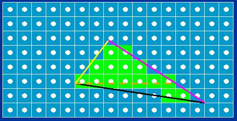
Figure 5: A standard software rasterization approach, used by Pixomatic 1, in which the triangle is rasterized as either one or two trapezoids. This triangle is subdivided into two trapezoids; first the yellow and pink edges are set up and stepped down to the dashed line to generate spans of covered pixels, and then the black edge is set up and the black and pink edges are stepped from the dashed line to the bottom of the triangle.

图例 5 : 一个标准的软件光栅化方法, 被 Pixomatic 1 所用. 该方法把三角形栅格化为一个或两个梯形. 图上的三角形被分为两个梯形; 首先从黄色边与粉丝边步进往下到虚线, 来生成区域内的像素点, 然后黑色边与粉色边以虚线开始, 步进到三角形最底部.

This approach was efficient for scalar code, but it just doesn't lend itself to vectorization. There were several other reasons this approach didn't suit Larrabee well (for example, it emits pixel-high spans, but for vectorized shading you want 4×4 blocks, both in order to generate 2-D texture gradients and because a square aspect ratio results in the highest utilization of the vector units), but the big one was that I just could never come up with a way to get good results out of vectorizing edge stepping.

这种方法对于标量代码很有效, 但是它对向量化没有帮助. 还有其它几个原因让这种方法不适合 Larrabee (比如, 它生成了大段的像素点, 但为了矢量底纹你需要 4×4 的块, 生成二维纹理梯度同理, 因为一个四边形面系数能最大化利用向量单元), 但最大的原因是我找不到一个方法来让向量化边步进得到一个好结果.

Sweep 光栅化 (扫描光栅化)

Another approach, often used by hardware, is sweep rasterization. An example of this is shown in Figure 6. Starting at a top vertex, a vector stamp of 4×4 pixels is swept left, then right, then down, and the process is repeated until the whole triangle has been swept. The edge equation is evaluated directly at each of the 16 pixels for each 4×4 block that's swept over.

另一种方法是扫描光栅化, 经常被用于硬件. 图例 6 显示了一个例子. 从三角形最上方顶点开始, 一个 4×4 的矢量标记往左扫描, 往右, 然后往下, 这过程一直重复直到扫描出整个三角形. 扫描到的 4×4 块的 16 个像素点直接求值边方程式.

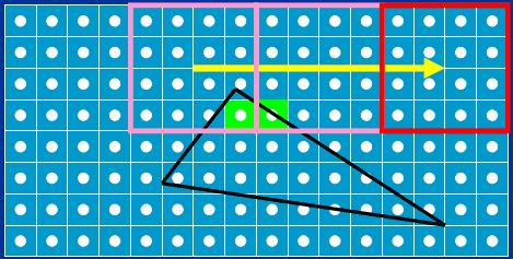
Figure 6: Sweep rasterization. Starting at the top vertex, a 4×4 pixel stamp is swept left until it's off the triangle, then right until it's off the triangle, and finally down, and then the process is repeated, until the whole triangle has been rasterized.

图例 6:扫描光栅化，从三角形最上方顶点开始, 一个 4×4 的矢量标记往左扫描直到离开三角形, 然后往右直到离开三角形, 然后往下, 这过程一直重复直到扫描出整个三角形.

Sweep rasterization is more vectorizable than the Pixomatic 1 approach, because evaluating the pixel stamp is well-suited to vectorization, but on the other hand it requires lots of badly-predicted branching, as well as a significant amount of work to decide where to descend. It also fails to take advantage of the ability of CPUs to make smart, flexible decisions, which was our best bet for being competitive with hardware rasterization, so we decided sweep rasterization wasn't the right answer.

扫描光栅化比　Pixomatic 1 方法更为可向量化, 因为标记像素点的求值很适合向量化, 但另一方面, 它需要很多强预测分支, 此外还需要一个重要的大量操作来决定从哪里往下扫描. 它也失败于利用 CPU 的有益功能来做漂亮灵活的判定, 这本是我们最确信可与硬件光栅化竞争的, 所以我们明白扫描光栅化也不是正确答案.

Larrabee 光栅化的一个上层视图

Larrabee takes a substantially different approach, one better suited to vectorization. In the Larrabee approach, we evaluate 16 blocks of pixels at a time to figure out which blocks are even touched by the triangle, then descend into each block that's at least partially covered, evaluating 16 smaller blocks within it, continuing to descend recursively until we have identified all the pixels that are inside the triangle. Here's an example of how that might work for our sample triangle.

Larrabee 采用了一个本质上不同的方法, 该方法更适合向量化. 在 Larrabee 方法中, 我们一次性求值 16 个块的像素点来找出那些块接触到三角形, 然后把每个部分覆盖三角形的块分为 16 个更小的块求值, 如此递归直到我们得到所有三角形内的像素点. 这里有个怎样运作起来的例子.

As I'll discuss shortly, the Larrabee renderer uses a chunking architecture. In a chunking architecture, the largest rasterization target at any one time is a portion of the render target called a tile; for this example, let's assume the tile is 64×64 pixels, as shown in Figure 7.

我接下来就会讲到, Larrabee 渲染器使用了程序分块架构. 在分块架构中, 任何一个时间最大的向量化对象是渲染对象的一部分, 称为一个瓦片(tile); 这个例子中, 我们假设一个瓦片是 64×64 像素点, 如图例 7 所示.

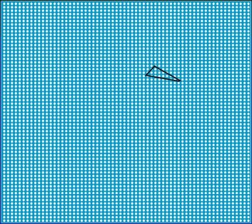
Figure 7: A triangle to be rasterized, shown against the pixels in a 64×64 tile.

图例 7 :一个要被光栅化的三角形，显示在 64×64 的瓦片中.

First, we test which of the 16×16 blocks (16 of them - we check 16 things at a time whenever possible, in order to leverage the 16-wide vector units) that make up the tile are touched by the triangle, as shown in Figure 8.

首先, 我们测定这瓦片中哪些 16×16 块( 16 个 - 我们尽可能一次性测定16个, 为了利用 16 宽的向量单元)碰触到三角形, 如图例 8 所示.

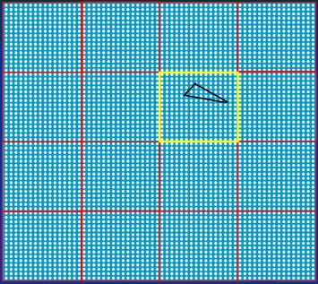
Figure 8: The 16 16×16 blocks are tested to see which are touched by the triangle.

图例 8 : 16 个 16×16 块被测定是否碰触到三角形.

We find that only one 16×16 block is touched, the block shown in yellow, so we descend into that block to determine exactly what is touched by the triangle, subdividing it into 16 4×4 blocks (once again, we check 16 things at a time to be vector-friendly), and evaluate which of those are touched by the triangle, as shown in Figure 9.

我们判定只有一个 16×16 块碰触到, 这个块显示为黄色, 所以我们进入这个块来更精确得判定, 把这个块分为 16 个 4×4 的块(再一次, 我们一次性判定 16 个, 对向量友好), 然后求值看哪些碰触到三角形, 如图 9 所示.

Figure 9: The 16 4×4 blocks are tested to see which are touched by the triangle.

图例 9 : 16 个 4×4 的块被判定是否碰触到三角形.

We find that 5 of the 4x4s are touched, so we process each of them separately, descending to the pixel level to generate masks for the covered pixels. The pixel rasterization for the first block is shown in Figure 10.

我们判定其中 5 个 4×4 块碰触到, 然后我们对他们每一个分别处理, 向下到像素点级别来标记包括在三角形里的像素点. 图例 10 显示第一个块的像素点光栅化.

Figure 10: Rasterization of the pixels in the first 4×4 block touched by the triangle.

图例 10 : 被三角形碰触到的第一个 4×4 块的像素点光栅化

Figure 11 shows the final result.

图例 11 显示最终结果.

Figure 11: All 5 4×4 blocks touched by the triangle have been rasterized.

图例 11 : 5 个三角形碰触到的 4×4 块都被光栅化后.

As you can see, the Larrabee approach processes 4×4 blocks, like the sweep approach, but unlike the sweep approach it doesn't have to make many decisions in order to figure out which blocks are touched by the triangle, thanks to the single 16-wide test performed before each descent. Consequently, this rasterization approach typically does somewhat less work than the sweep approach to determine which 4×4 blocks to evaluate. The real win, however, is that it takes advantage of CPU smarts by not-rasterizing whenever possible. I'll have to walk through the Larrabee rasterization approach in order to explain what that means, but as an introduction, let me tell you another optimization story.

如你所见, Larrabee 方法处理 4×4 块时, 很像扫描光栅化, 但与之不同的是它不需要进行很多判断来决定哪些块被三角形碰触到, 因为在每次之前都做过 16 宽的判定.因此, 比起扫描光栅化要求值哪些4×4块, 这种光栅化方法典型地减少了某种程度的工作量. 然而真正的胜利是, 它利用了 CPU 的优点来尽可能得非光栅化. 我将会详述 Larrabee 光栅化方法来解释, 但作为一个引言介绍, 让我先告诉你们另一个关于优化的故事.

Many years ago, I got a call from a guy I had once worked for. He wanted me to do some consulting work to help speed up his new company's software. I asked him what kind of software it was, and he told me it was image processing software, and that the problem lay in the convolution filter, running on a Sparc processor. I told him I didn't know anything about either convolution filters or Sparcs, so I didn't think I could be of much help, but he was persistent, so I finally agreed to take a shot at it.

很多年前, 我接到一个前老板的电话, 他希望我做些顾问工作来帮忙加速他新公司的软件. 我问他是哪种类型的软件, 他告诉我这是个图像处理程序, 问题出在回旋滤波器, 运行在 Sparc 处理器. 我告诉他对于回旋滤波器与 Sparcs 都不了解, 我不认为能提供多少帮助, 但他坚持, 所以我最终同意看看它.

He put me in touch with the engineer who was working on the software, who immediately informed me that the problem was that the convolution filter involved a great many integer multiplies, which the Sparc did very slowly, since at the time it didn't have a hardware integer multiply instruction. Instead, it had a partial product instruction, which had to be executed for each significant bit in the multiplier. In compiled code, this was implemented by calling a library routine that looped through the multiplier bits, and that routine was where all the time was going.

他让我和该软件的一个工程师联络, 该工程师立即告诉我问题出在回旋滤波器牵涉到大量整数乘法运算, 而 Sparc 对这些运算很慢, 因为那时 Sparc 还没有整数乘法硬件指令. 相反, 它有一个偏微商乘积指令, 得对乘数的每个信号位进行操作. 在编译后的代码中, 实现为调用一个位乘法的库循环, 该循环会一直运行.

I suggested unrolling that loop into a series of partial product instructions, and jumping into the unrolled loop at the right point to do as many partial products as there were significant bits, thereby eliminating all the loop overhead. However, there was still the question of whether to make the pixel value or the convolution kernel value the multiplier; the smaller the multiplier, the fewer partial products would be needed, so we wanted to pick whichever of the two was smaller, on average.

我建议展开那个循环为一连串偏微指令, 然后进入展开后的循环, 在恰当的点来处理尽可能多的偏微商乘积来处理信号位, 从而消除所有循环开销. 然而, 还是有问题在于是让像素点值还是让卷积内核值进行乘法.乘法越少, 所需偏微商乘积越少, 所以我们希望查看这两哪个更少, 或是差不多.

When I asked which was smaller, though, the engineer said there was no difference. When I persisted, he said they were random. When I said that I doubted they were random, since randomness is actually hard to come by, he grumbled. I don't know why he was reluctant to get me that information - I guess he thought it was a waste of time - but finally he agreed to gather the data and call me back.

当我询问哪个更少时, 那工程师却说没什么两样. 当我坚持询问, 他说它们是随机的. 我说我很怀疑它们是否随机, 因为很难得出随机量, 他开始发牢骚. 我不知道为何他不情愿让我得到那个信息 - 我猜他觉得是浪费时间 - 不过最后他同意收集数据并告诉我.

He didn't call me back that day, though. And he didn't call me back the next day. When he hadn't called me back the third day, I figured I might as well get it over with, and called him. He answered the phone, and, when I identified myself, he said, “Oh, hi. I'm just standing here with my managers, watching. We're all really happy.”

然而当天他并没通知我, 第二天也没有. 第三天还没通知我, 我感觉我要赶快把事情搞完, 打了电话给他. 他接了电话, 当我说明身份, 他说, “哦, 嗨. 我刚和我经理坐在一起看着, 我们都很高兴”

When I asked what exactly he was happy about, he replied, “Well, when I looked at the data, it turned out 90% of the values in the convolution kernel were zero, so I just put an if-not-zero around the multiply, and now the whole program runs three times faster!”

当我问他为何高兴, 他回复, “哦, 当我查看那些数据, 原来卷积核里有 90% 的值都是零, 所以我仅仅在乘法里做了一个非零判断, 现在程序就加速了三倍!”

Not-rasterizing is a lot like that, as we'll see shortly.

非光栅化也很类似这个, 我们很快就会看到.

瓦片(Tile)的分配

As noted earlier, Larrabee uses chunked (also known as binned or tiled) rendering, where the target is divided into multiple rectangles, called tiles. The rendering commands are sorted according to the tiles they touch and stored in the corresponding bins, and then the contents of each bin are rendered separately to the corresponding tile. It's a bit complex, but it considerably improves cache coherence and parallelization.

之前提到, Larrabee 使用块渲染, 把目标分成多个四边形, 称为瓦片(Tile). 渲染指令按瓦片被碰触的情况来排序,并存储到相应容器, 然后每个容器的指令分别执行渲染相应的瓦片. 这有点复杂, 但它改进了缓冲的一致性与并行性.

For chunking, rasterization consists of two steps; the first identifies which tiles a triangle touches, and the second rasterizes the triangle within each tile. So it's a two-stage process, and I'm going to discuss the two stages separately.

对于分块, 光栅化由两步组成; 第一步确认哪些瓦片碰触到三角形, 第二步对每个瓦片进行光栅化. 所以这个过程有两个阶段, 我将会分开讨论这两个阶段.

Figure 12 shows an example of a triangle to be drawn to a tiled render target. The light blue area is a 256×256 render target, subdivided into four 128×128 tiles.

图例 12 显示了一个三角形将被画到一个瓦片的例子. 亮蓝色区域是 256×256 的渲染对象, 被分成四个 128×128 的瓦片.

Figure 12: A triangle to be drawn to a 256×256 render target consisting of four 128×128 tiles.

图例 12 : 一个三角形要被画到由四个 128×128 瓦片组成的 256×256 渲染对象上.

With Larrabee's chunking architecture, the first step in rasterizing the triangle in Figure 12 is to determine which tiles the triangle touches, and put the triangle in the bins for those tiles, tiles 1 and 3. Once all triangles have been binned, the second step, intra-tile rasterization, is to rasterize the triangle to tile 1 when the tile 1 bin is rendered, and to rasterize the triangle to tile 3 when the tile 3 bin is rendered.

对于 Larrabee 的分块架构, 光栅化图例 12 三角形的第一步是判定哪些瓦片碰触到三角形, 然后把三角形数据放到这些瓦片容器里. 所有三角形都放置完毕后, 第二步就到瓦片内部进行光栅化, 当瓦片 1 被渲染时进行光栅化瓦片 1 中的三角形, 当瓦片 3 被渲染时光栅化 瓦片 3 中的三角形.

Assignment of triangles to tiles can easily be performed for relatively small triangles - say, up to a tile in size, which covers 90% of all triangles - by doing bounding box tests. For example, it would be easy with bounding box tests to find out what two tiles the triangle in Figure 12 is in. Larger triangles are currently assigned to tiles by simply walking the bounding box and testing each tile against the triangle; that doesn't sound very efficient, but tile-assignment time is generally an insignificant part of total rendering time for larger triangles, since there's usually a lot of shading work and the like to do for those triangles. However, if large-triangle tile assignment time does turn out to be significant, we could use a sweep approach, as discussed earlier, or a variation of the hierarchical approach used for intra-tile rasterization, which I'll discuss next. This is a good example of how a CPU makes it easy to use two completely different approaches in order to do the 90% case well and the 10% case adequately (or well, but in a different way), rather than having to have one size fit all.

通过使用盒包围测试能让相对小的三角形易分配到瓦片 - 所谓相对小是瓦片大小能达到覆盖三角形的90% . 例如, 很容易使用盒包围测试来找出图例 12 中三角形在哪两个瓦片中. 更大的三角形的分配是移动盒包围与测定每个瓦片相对三角形位置; 这听起来不怎么有效率, 但瓦片分配时间在整个大三角形渲染中通常微不足道. 然而, 如果大三角形瓦片分配时间比重变大, 我们可以使用之前提到的扫描法, 或者使用瓦片内部光栅化的分级方法的变种, 这之后会讨论到. 这是个好例子, 来看 CPU 怎么方便地使用两种完全不同的方法来干好 90% 的情况并适当处理(或是做好, 用另一种办法)剩余 10% 的情况, 而不是只能采用一种方法来通用处理.

Large-triangle assignment to tiles is performed with scalar code, for simplicity and because it's not a significant performance factor. Let's look at how that scalar process works, because it will help us understand vectorized intra-tile rasterization later. I'll use a small triangle for the example, for simplicity and to make the figures legible, but as noted above, normally such a small triangle would be assigned to its tile or tiles using bounding box tests.

大三角形的瓦片分配使用标量代码执行, 因为简单而且它不是性能的重要因素. 让我们看看标量过程是怎么工作的, 这会帮助我们理解之后的瓦片内光栅化的向量化. 为了让图例简单易懂, 我将使用一个小三角形的例子, 但如上面提到过的, 正常情况下小三角形是用盒包围测试来分配瓦片的.

Once we've set up the equation for an edge (by calculating B and C, as discussed when we looked at Figure 1), the first thing we do is calculate its value at the trivial reject corner of each tile. The trivial reject corner is the corner at which an edge's equation is most negative within a tile; the selection of the trivial reject corner for a given edge is based on its slope, as we'll see shortly. We set things up so that negative means inside in order to allow us to generate masks directly from the sign bit, so you can think of the trivial reject corner as the point in the tile that's most inside the edge. If this point isn't inside the edge, no point in the tile can be inside the edge, and therefore the whole triangle can be ignored for that tile.

当我们建立三角形一条边的方程式后( 计算 B 和 C 系数, 如图例 1 我们所讨论的), 我们做的第一件事是计算每个瓦片的平凡拒绝角的值. 平凡拒绝角就是瓦片里该边方程式值最小的角; 该边的平凡拒绝角的选择基于边的斜率, 我们很快就会看到. 前面我们已经确立了负值意味着在内部以方便直接遮罩标志位, 所以你可以认为一个瓦片的平凡拒绝角是该瓦片在该条边上最内部的点. 如果这个点不在该边内部, 那么就该瓦片就没有点在该边内部, 因此该瓦片就可以忽略整个三角形.

Figure 13 shows the trivial reject test in action. Tile 0 is trivially rejected for the black edge and can be ignored, because its trivial reject corner is positive, and therefore the whole tile must be positive and must lie outside the triangle, while the other three tiles must be investigated further. You can see here how the trivial reject corner is the corner of each tile most inside the black edge; that is, the point with the most negative value in the tile.

图例 13 显示了测定平凡拒绝角的手法. 瓦片 0 被黑边平凡拒绝, 可以忽略, 因为它的平凡拒绝角是正的值, 因此整个瓦片肯定都是正的,位于三角形之外, 而另外三个瓦片则需要进一步研究. 这里你可以看到平凡拒绝角是每个瓦片在黑边最内部的角; 即瓦片上值最小的点.

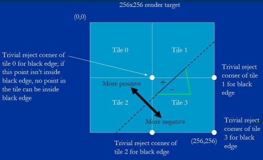
Figure 13: The tile trivial reject test.

图例 13 瓦片平凡拒绝角的测定.

Note that which corner is the trivial reject corner will vary from edge to edge, depending on slope. For example, it would be the lower left corner of each tile for the edge shown in red in Figure 14, because that's the corner that's most inside that edge.

注意哪个角是平凡拒绝角会随着边变化, 取决于边斜率. 比如, 图例 14 中红边的平凡拒绝角是各个瓦片的坐下角, 因为这是该边最内部的角.

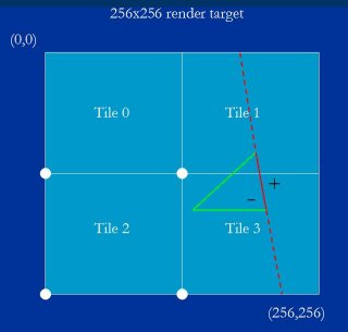
Figure 14: Which corner is the trivial reject corner varies with edge slope. Here the lower left corner of each tile is the trivial reject corner.

图例 14 : 平凡拒绝角随边斜率而改变, 这里各个瓦片的平凡拒绝角是左下角.

If you understand what we've just discussed, you're ninety percent of the way to understanding the whole Larrabee rasterizer. The trivial reject test is actually very straightforward once you understand it - it's just a matter of evaluating the sign of a simple equation at the right point - but it can take a little while to get it, so you may find it useful to re-read the previous section if you're at all uncertain or confused.

如果你理解了刚才我们所讨论的, 你就能理解整个 Larrabee 光栅化的百分之九十. 平凡拒绝角测试是很直接的, 只要你理解了它 - 它仅是关于对适当的点进行方程式求值的问题 - 但理解它需要花费一些时间, 如果你还是很困惑, 重读一遍前面内容会很有用.

So that's the tile trivial reject test. The other tile test is the trivial accept test. For this, we take the value at the trivial reject corner (the corner we just discussed) and add the amount that the edge equation changes for a step all the way to the diagonally opposite tile corner, the tile trivial accept corner. This is the point in the tile where the edge equation is most positive; you can think of this as the point in the tile that's most outside the edge. If the trivial accept corner for an edge is negative, that whole tile is trivially accepted for that edge, and there's no need to consider that edge when rasterizing within the tile.

这就是平凡拒绝角测验. 另一个瓦片测验是平凡接受测验. 这个测验从获取平凡拒绝角((刚讨论过的)边方程式的值转变成获取该瓦片对角的, 即平凡接受角. 这是瓦片上边方程式值最大的点; 你可以认为是该瓦片上离该边最外部的点. 如果该边的平凡接受角是负的, 那么整个瓦片被该边平凡接受, 那么就没必要在该瓦片光栅化时考虑这条边了.

Figure 15 shows the trivial accept test in action. Since the trivial accept corner is the corner at which the edge's equation is most positive, if this point is negative - and therefore inside the edge - all points in the tile must be inside the edge. Thus, tiles 0 and 1 are not trivially accepted for the black edge, because the equation for the black edge is positive at their trivial accept corners, but tiles 2 and 3 are trivially accepted, so rasterization of this triangle in tiles 2 and 3 can ignore the black edge entirely, saving a good bit of work.

图例 15 显示了如何测验平方接受角. 由于平凡接受角是边方程式值最大的角, 如果这个点是负值 - 因此在该边内部 - 那么该瓦片所有点肯定都在该边内部. 这样, 瓦片 0 和 1 不被黑边平凡接受, 因为它们的平凡接受角的黑边方程式值是正的, 但瓦片 2 和 3 被平凡接受, 那么瓦片 2 和 3 的光栅化就可以忽略整条黑边, 节省了好一些工作量.

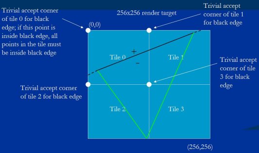
Figure 15: The tile trivial accept test.

图例 15 : 平凡接受角测验.

There's an important asymmetry here. When we looked at trivial reject, we saw that it applies to the whole triangle in the tile being drawn to, in the sense that trivially rejecting a tile against any edge means the triangle doesn't touch that tile, and so the triangle can be ignored in that tile. However, trivial accept applies only to the edge being checked; that is, trivially accepting a tile against an edge only means that specific edge doesn't have to be checked when rasterizing the triangle to that tile, because the whole tile is inside that edge; it has no direct implication for the whole triangle. The tile may be trivially accepted against one edge, but not against the others; in fact, it may be trivially rejected against one or both of the other edges, in which case the triangle won't be drawn to the tile at all. This is illustrated in Figure 16, where tile 3 is trivially accepted against the black edge, so the black edge wouldn't need to be considered in rasterizing the triangle to that tile, but tile 3 is trivially rejected against the red edge, and that means that the triangle doesn't have to be rasterized to tile 3 at all.

这里有个重要的不对等. 当我们看平凡拒绝, 我们发现它应用于整个三角形, 意味着任意边的平凡拒绝都意味整个三角形都不碰触该瓦片, 该瓦片可忽略整个三角形. 然而, 平凡接受只应用于所测验的边; 也就是, 一条边平凡接受一个瓦片只意味着该边在该瓦片光栅化时可不被检查, 因为整个瓦片都在该边内部; 对整个三角形而言则没有直接意义. 一个瓦片可能被一条边平凡接受(译者: 此处作者可能有笔误), 但这不意味着被其它边平凡接受; 实际上, 它可能被一条或两条边平凡拒绝, 这种情况就是三角形不会画在该瓦片上. 图 16 有说明, 瓦片 3 被黑边平凡接受, 这样在光栅化三角形到该瓦片时就没必要考虑黑边, 但瓦片 3 被红边平凡拒绝, 这意味着三角形不需要在瓦片 3 中光栅化.

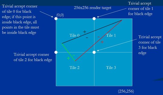
Figure 16: Tile 3 is trivially accepted against the black edge, but trivially rejected against the red edge.

图例 16 :瓦片 3 被黑边平凡接受, 但被红边平凡拒绝.

In Figure 17, however, tile 3 is trivially accepted by all three edges, and here we come to a key point.

然而在图例 17 中, 瓦片 3 被三条边平凡接受, 这里有个关键点.

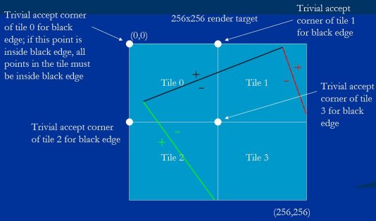
Figure 17: Tile 3 is trivially accepted against all three edges.

图例 17 :瓦片 3 被三条边平凡接受.

If all three edges are negative at their respective trivial accept corners, then the whole tile is inside the triangle, and no further rasterization tests are needed - and this is what I meant earlier when I said the rasterizer takes advantage of CPU smarts by not-rasterizing whenever possible. The tile-assignment code can just store a draw-whole-tile command in the bin, and the bin rendering code can simply do the equivalent of two nested loops around the shaders, resulting in a full-screen triangle rasterization speed of approximately infinity - one of my favorite performance numbers!

如果三条边各自的平凡接受角都是负值, 那么整个瓦片都在三角形内部, 就不需要进一步光栅化了 - 这就是我之前所说的利用 CPU 的优势来尽可能的非光栅化. 瓦片分配的代码可以仅仅储存一个“画整个瓦片”的命令在容器里, 容器渲染代码可以简单做两个渲染器的嵌套循环, 结果是无限接近于全屏三角形光栅化的速度 - 我最爱的性能数字之一.

By the way, this whole process should be familiar to 3-D programmers, because testing of bounding boxes against planes (for example, for frustum culling) is normally done in exactly the same way - although in three dimensions instead of two - with the same use of sign to indicate inside and outside for trivial accept and reject. Also, structures such as octrees employ a 3-D version of the hierarchical recursion used by the Larrabee rasterizer..

顺便一提, 3D 程序员应该对这整个过程比较熟悉, 因为平面盒包围测试(比如圆锥截取)通常使用相同的方法 - 虽然是三维取代了二维 - 同样使用了标记平凡拒绝与平凡接受来区分内部与外部. 同样, 八叉树的架构使用了 3D 版本的Larrabee 光栅器分层递归.

That completes our overview of how rasterization of large triangles for tile assignment works. As I said, this is done as a scalar evaluation in the Larrabee pipeline, so the trivial accept and reject tests for each tile are performed separately. Intra-tile rasterization, to which we turn next, is much the same, but vectorized, and it is this vectorization that will give us insight into applying the Larrabee New Instructions to semi-parallel tasks.

这就是完整的大三角形瓦片分配的概况. 如我所说, 在 Larrabee 处理管道中这些是作为标量来计算的, 所以每个瓦片的平凡接受与平凡拒绝测验是分开执行的. 我们接下来讲的瓦片内光栅化, 也很类似, 但它要被向量化, 这些向量化可以让我们理解怎么在半并行化任务上应用 Larrabee 新指令集.

Intra-tile rasterization starts at the level of a whole tile. Tile size varies, depending on factors such as pixel size, but let's assume that we're working with a 64×64 tile. Given that starting size, we calculate the edge equation values at the 16 trivial reject and trivial accept corners of the 16×16 blocks that make up the tile, just as we did at the tile level - but now we do these calculations 16 at a time. Let's start with the trivial reject test.

瓦片内光栅化先从整个瓦片级别开始. 瓦片尺寸是可变的,取决于像素点尺寸等因素, 但我们先假设处理的瓦片是 64×64. 从这个尺寸, 我们计算组成瓦片的 16 个块的平凡拒绝角与平凡接受角, 和我们之前在瓦片级别干的一样 - 但是现在我们是同时计算 16 个. 让我们先开始平凡拒绝测验.

First, we calculate which corner of the tile is the trivial reject corner, calculate the value of the edge equation at that point, and set up a table containing the 16 steps of the edge equation from the value at the tile trivial reject corner to the trivial reject corners of the 16×16 blocks that make up the tile. The signs of the 16 values that result tell us which of the blocks are entirely outside the edge, and can therefore be ignored, and which are at least partially accepted, and therefore have to be evaluated further.

首先, 我们计算哪个角是瓦片的平凡拒绝角, 并计算该点的边方程值, 然后建立一个表,以瓦片平凡拒绝角的值来步进以获得包括 16 个组成瓦片的块的平凡拒绝角的边方程式值. 16 个结果值的正负号告诉我们哪些块完全在边外部也就是能被忽略, 以及哪些块至少部分被接受,因此需要进一步评估.

In Figure 18, for example, we calculate the trivial reject values for the black edge, by stepping from the value we calculated earlier at the trivial reject corner of the tile, and eliminate five of the 16×16 blocks that make up the tile. The trivial reject corner for the tile is shown in red, and the 16 trivial reject corners for the blocks are shown in white. The gray blocks are the ones that are rejected against the black edge; you can see that their trivial reject corners all have positive edge equation values. The other 11 blocks have negative values at their trivial reject corners, so they're at least partially inside the black edge.

图例 18 中, 举个例子, 我们从先前计算出的瓦片的平凡拒绝角的值来步进获取黑边的块平凡拒绝角的值, 然后在组成瓦片的 16×16 块中去除了其中 5 个. 瓦片的平凡拒绝角显示为红色, 16 个块平凡拒绝角则显示为白色. 灰色块即被黑边拒绝的; 你可以看到它们的平凡拒绝角的边方程式值都是正的. 另外 11 个块的平凡拒绝角则是负值, 所以他们至少是部分在黑边内部.

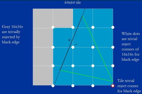
Figure 18: The trivial reject tests for the 16 16×16 blocks in the tile.

图例 18 : 瓦片 16×16 个块的平凡拒绝角的测验.

To make this process clearer, in Figure 19 the arrows represent the 16 steps that are added to the black edge's tile trivial reject value. Each of these steps is just an add, and we can do 16 adds with a single vector instruction, so it takes only one vector instruction to generate the 16 trivial reject values, and one more vector instruction - a compare - to test them.

为了让这个过程更为清晰, 在图例 19 中展示了 19 个箭头到瓦片的黑边平凡拒绝角, 显示 16 个值的步进. 其中每个步进只是一个加法, 我们可以在一个向量结构中一次处理 16 个加法, 所以获取 16 个平凡拒绝角的值只需要做一个向量结构, 和另一次向量结构 - 用于比较 - 来测验.

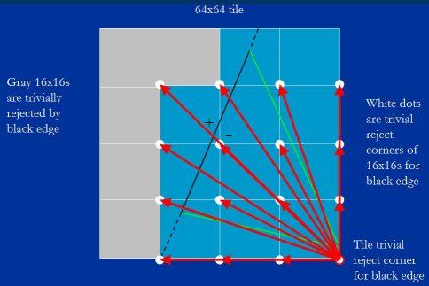
Figure 19: The steps from the tile trivial reject corner for the black edge to the trivial reject corners of the 16 16×16 blocks for the black edge.

图例 19:　瓦片黑边平凡拒绝角到 16 个块的黑边平凡拒绝角的步进.

All this comes down to just setting up the right values, then doing one vector add and one vector compare. Remember that the edge equation is of the form Bx + Cy; therefore, to step a distance across the tile, we just set x and y to the horizontal and vertical components of that distance, evaluate the equation, and add that to the starting value. So all we're doing in Figure 19 is adding the 16 values that step the edge equation to the 16 trivial reject corners. For example, to get the edge equation value at the trivial reject corner of the upper-left block, we'd start with the value at the tile trivial reject corner, and add the amount that the edge equation changes for a step of -48 pixels in x and -48 pixels in y, as shown by the yellow arrow in Figure 20. To get the edge equation value at the trivial reject corner of the lower-left block, we'd instead add the amount that the edge equation changes for a step of -48 pixels in x only, as shown by the purple arrow. And that's really all there is to the Larrabee rasterizer - it's just a matter of stepping the edge equation values around the tile so as to determine what blocks and pixels are inside and outside the edges.

所有这些归结为只要建立对应的值, 然后做一次向量加法与一次向量比较. 记得边方程式的形式是 Bx + Cy; 因此, 在瓦片上的步进, 可以把 x 和 y 设为横竖相对距离, 然后求值, 并加上初始值. 所以图例 19 中我们所做的就是把 16 个步进值加到 16 个平凡拒绝角. 比如, 为了得到左上角块的平凡拒绝角的边方程式值, 我们会从瓦片的平凡拒绝角的值开始, 加上 x 为 -48 及 y 为 -48 的边方程式的值, 如图例 20 中的黄色箭头. 为了得到左下角块的平凡拒绝角的值, 我们则加上 x 为 -48 及 y 为 0 的边方程式值, 如紫色箭头所示. 这就是 Larrabee 光栅化真正所有的 - 它就是步进这些边方程式值来决定哪些块和像素点是在边的外部还是内部.

Figure 20: Examples of stepping the edge equation Bx + Cy.

图例 20 :　边方程式 Bx + Cy 的步进例子.

Once again, we'll do trivial accept tests as well as trivial reject tests. In Figure 21 we've calculated the trivial accept values, and determined that 6 of the 16×16 blocks are trivially accepted for the black edge, and 10 of them are not trivially accepted. We know this because the values of the equation of the black edge at the trivial accept corners of the 6 pink blocks are negative, so those blocks are entirely inside the edge, while the values at the trivial accept corners of the other 10 blocks are positive, so those blocks are not entirely inside the black edge. The trivial accept values for the blocks can be calculated by stepping in any of several different ways: from the tile trivial accept corner, from the tile trivial reject corner, or from the 16 trivial reject values for the blocks. Regardless, it again takes only one vector instruction to step and one vector instruction to test the results. Combined with the results of the trivial reject test, we also know that 5 blocks are partially accepted.

再次, 我们会像平凡拒绝角那样来做平凡接受角测验. 在图例 21 中我们已经计算出这些平凡接受角的值, 并判定 其中 6 个 16×16 的块是被黑边平凡接受的, 另外 10 个则不被平凡接受. 我们知道这是因为那 6 个粉丝块的黑边平凡接受角的值是负的, 那么这些块整体都在该边的内部; 而另外 10 个块的平凡接受角值是正的, 那么它们不是整体处于黑边内部. 这些块的平凡接受角的值的计算可以使用几种方法来步进:　从瓦片的平凡接受角来步进, 从瓦片的平凡拒绝角来步进, 或从 16 个平凡拒绝角的值来步进. 不管怎样, 这再次只耗费一次向量结构来步进与一次向量结构来测验. 结合平凡接受角的测验, 我们也知道有 5 个块被部分接受.

Figure 21: The trivial accept tests for the 16 16×16 blocks in the tile.

图例 21 : 瓦片上 16 个 16×16 的块的平凡接受角测验.

The 16 trivial reject and trivial accept values can be calculated with a total of just two vector adds per edge, using tables generated at triangle set-up time, and can be tested with two vector compares, which generate mask registers describing which blocks are trivially rejected and which are trivially accepted. We do this for the three edges, ANDing the results to create masks for the triangle, do some bit manipulation on the masks so they describe trivial and partial accept, and bit-scan through the results to find the trivially and partially accepted blocks. Each 16×16 that's trivially accepted against all three edges becomes one bin command; again, no further rasterization is needed for pixels in trivially accepted blocks.

通过三角形建立时生成的表, 每个边的 16 个平凡拒绝和平凡接受的值可以仅由两次向量加法来计算, 并由两次向量比较来测验, 生成标记寄存器来标识哪些块被平凡拒绝哪些被平凡接受. 我们执行三条边, 生成建立三角形的标识, 在这些标识上做些位操作来表示被平凡拒绝或平凡接受, 之后通过结果的位扫描可以找出被平凡拒绝和平凡接受的块. 每个 16×16 的被三条边平凡接受的会转为一个二进制命令 再次, 被平凡接受的块不需要进一步光栅化.

This is not obvious stuff, so let's take a moment to visualize the process. First, let's just look at one edge and trivial accept.

这并不怎么明显, 所以让我们花一些时间来对这过程有个印象. 首先, 我们只看一条边和平凡接受.

For a given edge, say edge number 1, we take the edge equation value at the tile trivial accept corner, broadcast it out to a vector, and vector add it to the precalculated values of the 16 steps to the trivial accept corners of the 16×16 blocks. This gives us the edge 1 values at the trivial accept corners of the 16 blocks, as shown in Figure 22. (The values shown are illustrative, and are not taken from a real triangle.)

对给定边, 称为边 1, 我们取得瓦片平凡接受角的该边方程式的值, 广播给一个向量处理器(阵列处理器),阵列处理器把它加到预先计算好的 16×16 块的步进值. 这就给了我们 16 个块的边 1 平凡接受角的值. 如图 22. ( 显示的值是用过说明的, 所以不是取自真实三角形)

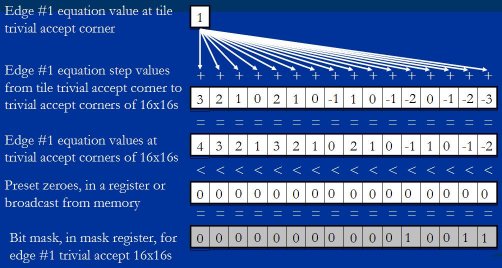
Figure 22: Edge 1 trivial accept tests for the 16 16×16 blocks.

图 22 : 16 个 16×16 块的边 1 的平凡接受测验.

The step values shown on the second line in Figure 22 are computed when the triangle is set up, using a vector multiply and a vector multiply-add. At the top level of the rasterizer - testing the 16×16 blocks that make up the tile, as shown in Figure 22 - those set-up instructions are just direct additional rasterization costs, since the top level only gets executed once per triangle, so it would be accurate to add 6 instructions to the cost of the 16×16 code we'll look at shortly in Listings 1 and 2. However, as the hierarchy is descended, the tables for the lower levels (16×16-to-4×4 and 4×4-to-mask) get reused multiple times. For example, when descending from 16×16 to 4×4 blocks, the same table is used for all partial 16×16 blocks in the tile. Likewise, there is only one table for generating masks for partial 4×4 blocks, so the additional cost per iteration in Listing 3 due to table set-up would be 2 instructions divided by the number of partial 4×4 blocks in the tile. This is generally much less than 1 instruction per 4×4 block per edge, although it gets higher the smaller the triangle is.

Then we compare the results to 0; as shown in Figure 22, this generates a mask that contains 1-bits where a block trivial accept corner is less than zero - that is, wherever a block trivial accept corner is inside the edge, meaning the whole block is inside the edge.

We do this for each of the three edges, ANDing the masks together to produce a composite mask, as shown in Figure 23. (The ANDing happens automatically as part of the mask updating, as we'll see later when we look at the code.) This composite mask has 1-bits only where a block trivially accepts against all three edges, which is to say for blocks that are fully trivially accepted and require no further rasterization.

Figure 23: Generating the composite trivial accept mask for the three edges.

Now we can bit-scan through the composite mask, picking out the 16×16 blocks that are trivially accepted, and storing a draw-block command for each of them in the rasterizer output queue. The first bit-scan would find that block 0 is trivially accepted, the second bit-scan would find that block 4 is trivially accepted, and the third bit-scan would find that there were no more trivially accepted blocks, as shown in Figure 24.

Figure 24: Scanning through the composite trivial accept mask to find trivially accepted 16×16 blocks.

This sort of parallel-to-serial conversion - identifying and processing relevant elements of a vector result efficiently - is key to getting good performance out of semi-vectorizable code. This is exactly why the bsfi instruction was added as part of the Larrabee New Instructions. Bsfi is based on the existing bit-scan instruction but is enhanced to allow starting the scan at any bit, rather than only at bit 0.

We're finally ready to look at some real code. Listing 1 shows just the trivial accept code for the 16×16 blocks in a 64×64 tile; this will suffice to illustrate what we've discussed, and anything more would just complicate the explanation. Let's map these instructions to the steps we just described.

; On entry:
; rsi: base pointer to thread data
; v3: steps from edge 1 tile trivial accept corner to corners of 16x16 blocks
; v4: steps from edge 2 tile trivial accept corner to corners of 16x16 blocks
; v5: steps from edge 3 tile trivial accept corner to corners of 16x16 blocks

; Step to edge values at 16 16x16 block trivial accept corners
vaddpi v0, v3, [rsi+Edge1TileTrivialAcceptCornerValue]{1to16}
vaddpi v1, v4, [rsi+Edge2TileTrivialAcceptCornerValue]{1to16}
vaddpi v2, v5, [rsi+Edge3TileTrivialAcceptCornerValue]{1to16}

; See if each trivial accept corner is inside all three edges
; K1 is set by the first instruction, then the result of the
; second instruction is ANDed with k1, and likewise for the third instruction
vcmpltpi k1, v0, [rsi+ConstantZero]{1to16}
vcmpltpi k1{k1}, v1, [rsi+ConstantZero]{1to16}
vcmpltpi k1{k1}, v2, [rsi+ConstantZero]{1to16}

; Get the mask; 1-bits are trivial accept corners that are
; inside all three edges
kmov eax, k1

; Loop through 1-bits, issuing a draw-16x16-block command
; for each trivially accepted 16x16 block
bsf ecx, eax
jnz TrivialAcceptDone

TrivialAcceptLoop:
; <Store draw-16x16-block command, along with (x,y) location>

bsfi ecx, eax
jnz TrivialAcceptLoop
TrivialAcceptDone:

Listing 1: Trivial accept code for 16×16 blocks.

First, there are three vector adds to step the 3 edge values to the trivial accept corners of the 16x16s; these are the three vaddpi instructions.

Second, there are three vector compares to test the signs of the results, to see if the blocks are trivially accepted against the edges; these are the three vcmpltpi instructions. The composite mask is accumulated in mask register k1.

Next, the kmov copies the mask of trivially accepted blocks into register eax, and finally, there is a loop to bit-scan eax to pick out the trivially accepted 16x16s, one by one, so they can be processed as blocks, without further rasterization.

It takes only 6 vector instructions, one mask move, and two scalar instructions to set up, plus two scalar instructions per trivially accepted block, to find all the trivially accepted 16x16s in a tile.

And, in truth, it doesn't even take that many instructions. What's shown in Listing 1 is a version of the trivial accept code that uses normal vector instructions, but there's actually a special instruction specifically designed to speed up rasterization - vaddsetspi - that both adds and sets the mask to the sign. I haven't mentioned it because I thought the discussion would be clearer and more broadly relevant if I used the standard vector instructions, but as you can see in Listing 2, if we use vaddsetspi we need only 3 vector instructions to find all the trivially accepted 16×16 blocks.

; On entry:
; rsi: base pointer to thread data
; v3: steps from edge 1 tile trivial accept corner to corners of 16x16 blocks
; v4: steps from edge 2 tile trivial accept corner to corners of 16x16 blocks
; v5: steps from edge 3 tile trivial accept corner to corners of 16x16 blocks

; Step to edge values at 16 16x16 block trivial accept corners &
; see if each trivial accept corner is inside all three edges
kxnor k1, k1 ; set mask to 0xFFFF
; The result of each instruction is ANDed with k1
vaddsetspi v0 {k1}, v3, [rsi+Edge1TileTrivialAcceptCornerValue]{1to16}
vaddsetspi v1 {k1}, v4, [rsi+Edge2TileTrivialAcceptCornerValue]{1to16}
vaddsetspi v2 {k1}, v5, [rsi+Edge3TileTrivialAcceptCornerValue]{1to16}

; Get the mask; 1-bits are trivial accept corners that are
; inside all three edges
kmov eax, k1

; Loop through 1-bits, issuing a draw-16x16-block command
; for each trivially accepted 16x16 block
bsf ecx, eax
jnz TrivialAcceptDone

TrivialAcceptLoop:
; <Store draw-16x16-block command, along with (x,y) location>

bsfi ecx, eax
jnz TrivialAcceptLoop
TrivialAcceptDone:

Listing 2: Trivial accept code for 16×16 blocks using vaddsetspi.

There may also be fewer active edges due to trivial accepts at the tile level (remember, edges that are trivially accepted for a tile can be - and are - ignored when rasterizing within the tile), and that would result in still fewer instructions; this is another case in which software can boost performance by adapting to the data.

We're now done rasterizing trivially accepted 16×16 blocks, but we still have to handle partially-covered 16×16 blocks, and by this point it should be obvious how that works; we descend into each partial 16×16 to evaluate the 4×4 blocks it contains, just as we descended into the 64×64 tile to evaluate the 16x16s it contained. Again, we put trivially accepted 4x4s directly into the bin. Partially accepted 4x4s, however, need to be processed into pixel masks. This is done with a vector add of a precalculated, position-independent table for each edge that steps from the 4×4 trivial reject corner to the center of the pixel itself; the sign bits can then be ANDed together to form the pixel mask.

Figure 25 illustrates the calculation of the pixel mask. From the trivial-reject corner of the 4×4, shown in red, a single add yields the equation value for the black edge at the 16 pixel centers. The red arrows show how the 16 values in the precalculated, position-independent step table for each edge are added to the trivial reject corner of the 4×4 to evaluate the edge equation at the 16 pixel centers. The pixels shown in blue have negative values and are inside the edge. This slide shows the actual mask that is generated, with a 1-bit for each pixel inside the edge, and a 0-bit for each pixel that's outside.

Figure 25: The pixel mask is calculated at pixel centers by stepping relative to the trivial reject corner for the 4×4.

Figure 25 is a good demonstration of how vector efficiency can fall off with partially-vectorizable tasks, and why Larrabee uses 16-wide vectors rather than something larger. We will often do all the work needed to generate the pixel mask for a 4×4, only to find that many or most of the pixels are uncovered, so much of the work has been wasted - and the wider the vector, the lower the ratio of covered to uncovered becomes, on average, and the more work is wasted.

Listing 3 shows code for calculating the pixel masks for all the partially-covered 4×4 blocks in a partially-covered 16×16 block. Note that this is the only case in which per-pixel work is performed; all solidly-covered-block cases are handled without generating a pixel mask.

; On entry:
; rbx: pointer to output buffer
; rsi: base pointer to thread data
; k1: mask of partially accepted 4x4 blocks in the current 16x16
; v0: edge 1 trivial reject corner values for 4x4 blocks in the current 16x16
; v1: edge 2 trivial reject corner values for 4x4 blocks in the current 16x16
; v2: edge 3 trivial reject corner values for 4x4 blocks in the current 16x16

; Store values at corners of 16 4x4s in 16x16 for indexing into
vstored [rsi+Edge1TrivialRejectCornerValues4x4], v0
vstored [rsi+Edge2TrivialRejectCornerValues4x4], v1
vstored [rsi+Edge3TrivialRejectCornerValues4x4], v2

; Load step tables from corners of 4x4s to pixel centers
vloadd v3, [rsi+Edge1PixelCenterTable]
vloadd v4, [rsi+Edge2PixelCenterTable]
vloadd v5, [rsi+Edge3PixelCenterTable]

; Loop through 1-bits from trivial reject test on 16x16 block (trivial accepts have been
; XORed out earlier), descending to rasterize each partially-accepted 4x4
kmov eax, k1
bsf ecx, eax
jnz Partial4x4Done

Partial4x4Loop:
; See if each of 16 pixel centers is inside all three edges
; Use rcx, the index from the bit-scan of the current partially accepted 4x4, to index into
; the 4x4 trivial reject corner values generated at the 16x16 level, and pick out the
; trivial reject corner values for the current partially accepted 4x4
; K2 is set by the first instruction, then the result of the
; second instruction is ANDed with k2, and likewise for the third instruction
vcmpgtpi k2, v3, [rsi+Edge1TrivialRejectCornerValues4x4+rcx*4]{1to16}
vcmpgtpi k2 {k2}, v4, [rsi+Edge2TrivialRejectCornerValues4x4+rcx*4]{1to16}
vcmpgtpi k2 {k2}, v5, [rsi+Edge3TrivialRejectCornerValues4x4+rcx*4]{1to16}

; Store the mask
kmov edx, k2
mov [rbx], dx

; <Store the (x,y) location and advance rbx>

bsfi ecx, eax
jnz Partial4x4Loop
Partial4x4Done:

Listing 3: Pixel mask code for partially-covered 4×4 blocks.

Listing 3 first stores the trivial reject corner values for the 16 4×4 blocks for the three edges. These are the values we'll step relative to in order to generate the final pixel masks for each partial 4×4, and were generated earlier by the 16×16 code that ran just before this code. This is done with the three vstored instructions.

Next, the step tables for the three edges are loaded with the three vloadd instructions. (Actually, these will probably just be preloaded into registers when the triangle is set up and remain there throughout the rasterization of the triangle, but loading them here makes it clearer what's going on.)

Once that set-up is complete, the code scans through the partial accept mask, which was also generated earlier by the 16×16 code. First the mask is copied to eax with the kmov instruction, and then bsfi is used to find each partially-accepted 4×4 block in turn.

For each partially-covered 4×4 found, the code does three vector compares to evaluate the three edge equations at the 16 pixel centers. Note that each vcmpgtpi uses the index of the current 4×4 to retrieve the trivial reject corner value for that 4×4 from the vector generated at the 16×16 level. While we could directly add and then test the signs of the edge equations, as I described earlier, it's more efficient to instead rearrange the calculations by flipping the signs of the step tables so that the testing can be done with a single compare per edge. Put another way, instead of adding two values and seeing if the result is less than zero:

m + n < 0

it's equivalent and more efficient to compare one value directly to the negation of the other value:

m < -n.

(In case you're wondering, we couldn't use this trick at the 16×16 and 64×64 levels of the hierarchy because in those cases, in addition to getting the result of the test, we also need to keep the result of the add, so we can pass it down the hierarchy as the new corner value.)

The result of the compares is the final composite pixel mask for that 4×4, which can be stored in the rasterization output queue. And that's it: once things are set up, the cost to rasterize each partial 4×4 is three vector instructions, a mask instruction, and a handful of scalar instructions. Once again, if the whole tile was trivially accepted against one or two edges, then proportionately fewer vector instructions would be required.

One nice feature of the Larrabee rasterization approach is that MSAA - multisample antialiasing - falls out for one extra vector compare per 16 samples per edge, since it's just a different step from the trivial-reject corner. (That's for partially accepted 4×4 blocks; for all trivially accepted blocks, there is no incremental cost for rasterization of MSAA.) In Figure 26, each pixel is divided into four samples, and the step shown is to one of the four samples rather than to the center of each pixel; this takes one compare, so a total of four compares would be required to generate the full MSAA sample mask for 16 pixels.

Figure 26: Stepping to one set of samples for 4X MSAA rasterization of a partially-covered 4×4.

Now that we've stepped all the way down through the rasterization hierarchy, let's go back and look again at the rasterization descent overview we started with, this time with a detailed understanding what's going on.

Figure 27 shows a triangle and a 64×64 tile to which the triangle is to be drawn, with the tile subdivided into 16×16 blocks; Figure 27 is a repeat of Figure 8, but this time I've added dashed extensions of the edges to the border of the tile, so we can see what blocks and pixels are on what sides of the edges.

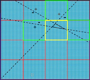
Figure 27: A triangle to be rasterized, shown against the pixels in a 64×64 tile. The 16×16 blocks that are not trivially rejected are highlighted in green and yellow.

To rasterize the triangle in Figure 27, we first calculate the values of the triangle's three edge equations at the tile's trivial accept and trivial reject corners, and find that the tile is neither trivially rejected nor trivially accepted by any edge. (Again, this would actually only be done for a large triangle; we would use bounding box tests for such a small triangle.) We set up the various step tables we'll use, and then we step the edge equations to their respective trivial accept and trivial reject corners of the 16 blocks, each 16×16 in size, that make up the tile, and make a mask containing the signs of the results.

We then bit-scan through the resulting mask, find that 12 of the 16 blocks are trivially rejected, and descend into each of the remaining 4 blocks in turn. In three of the blocks, we‘ll ultimately find that there's nothing to draw, so for the purposes of this discussion we'll ignore those and look at the more interesting case of what happens when we descend into the block that the triangle lies inside, the block outlined in yellow. (Note that if the triangle were large enough to fully cover a 16×16 block, that block would be trivially accepted, and no further descent into that block would be required.)

Before we look at what happens when we descend into the 16×16 block containing the triangle, there's one more thing in Figure 27 that we should take a look at. You may have noticed that in the earlier version of this figure, Figure 8, only the one block in yellow was found, not the three green blocks. Why did the bit-scan find 4 blocks this time, when the triangle is in fact entirely contained in one block? The reason is that the Larrabee rasterization approach, as discussed in this article, can only eliminate blocks by trivially rejecting them, and if you look closely, you will see that none of the three green blocks is trivially rejected by any edge. This is an inefficiency of this rasterization method, although there are techniques, which are beyond the scope of this article, that remove much of the inefficiency.

Descending the rasterization hierarchy, we take the 16×16 block containing the triangle, subdivide it into 16 4×4 blocks, and evaluate which of those are touched by the triangle by stepping to evaluate the edge equation at each of their trivial accept and trivial reject corners for each edge, as shown in Figure 28. We find that 10 of the blocks are trivially rejected, and that none of the 6 remaining blocks are trivially accepted against all three edges.

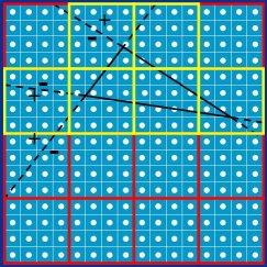
Figure 28: Rasterizing the sample triangle within the 16×16 block that contains it. The 4×4 blocks that are not trivially rejected are highlighted.

We've finally reached the bottom of the rasterization hierarchy, so we can bit-scan through the partial-accept mask generated for the 16×16, to find the partially-accepted 4×4 blocks, and generate the 4×4 pixel mask for each of the blocks in turn, as shown in Figure 29.

Figure 29: Rasterization of the pixels in the partial 4×4 blocks covering the triangle.

Here we see once again that the reliance on trivial reject to eliminate blocks has caused a false positive on a block that actually doesn't touch the triangle (the leftmost block). It's possible to do bounding box tests to eliminate such blocks, but it's not clear whether that's more efficient than just testing for empty masks - that is, masks with no pixels enabled - and skipping those blocks.

After completing this 16×16 block, we pop back up to rasterize the other 16×16 blocks that weren't trivially rejected (which in this case turned out not to contain any of the triangle).

And that's really all there is to it!

Now that we understand the basic rasterization algorithm, let's take a quick look at some interesting implementation refinements.

In software, we don't have the luxury of custom data and ALU sizes, but we do have the luxury of adapting to input data, and this adaptive rasterization helps boost our efficiency. For example, edge evaluations have to be done with 48 bits in the worst case; for those cases, being software, we have to use 64 bits, since there is no 48-bit integer support in Larrabee. However, we don't have to do that at all for the 90+% of all triangles that fit in a 128×128 bounding box, because in those cases 32 bits is enough.

When we do have to do 64-bit edge evaluation, we only have to use it for tile assignment. As it turns out, within tiles up to 128×128 in size (and 128×128 is our largest tile size), any edge that the tile's not trivially accepted or rejected against can always be rasterized using 32 bits.

We can also detect triangles that fit in a 16×16 bounding box, and process them with one less descent level, less set-up, and no trivial accept test (since there will rarely be trivially accepted 4x4s in such small triangles). Finally, triangles that fit in very small bounding boxes can be done simply by directly calculating the masks for the 16 or 32 pixels directly, with little set-up and minimal processing.

In fact, for small triangles we could even take the z value of the closest vertex and compare it to the z buffer for the triangle's bounding box, and possibly z-reject the triangle before we even rasterize it!

There are other optimization possibilities I won't get into because there's just not space in this article, and of course there's no telling how well they'll work until we try them, but one nice thing about software is that it's easy to run the experiments to check them out.

And with that, we conclude our lightning tour of the Larrabee rasterization approach, and our examination of how vector programming can be applied to a semi-parallel task. As I mentioned earlier, software rasterization will never match dedicated hardware peak performance and power efficiency for a given area of silicon, but so far it's proven to be efficient enough. It also has a significant advantage, which is that because it uses general purpose cores, the same resources that are used for rasterization can be used for other purposes at other times, and vice-versa. As Tom Forsyth puts it, because the whole chip is programmable, we can effectively bring more square millimeters to bear on any specific task as needed - up to and including the whole chip; in other words, the pipeline can dynamically reconfigure its processing resources as the rendering workload changes. If we get a heavy rasterization load, we can have all the cores working on it, if necessary; it wouldn't be the most efficient rasterizer per square millimeter, but it would be one heck of a lot of square millimeters of rasterizer, all doing what was most important at that moment, in contrast to a traditional graphics chip with a hardware rasterizer, where most of the circuitry would be idle when there was a heavy rasterization load. A little while later, when the load switches to shading, the whole Larrabee chip can become a shader if necessary. Software simply brings a whole different set of strengths and weaknesses to the table.

There's a lot to learn and rethink with Larrabee, and a lot of potential there. Only time will tell how well it all works out - but meanwhile, it certainly is an interesting time to be a performance programmer!

Further information about Larrabee is available at http://www.intel.com/software/graphics.